Integration of Control Lyapunov and Control Barrier Functions for Safety-Critical Guarantees in Aggregate Computing
Angela Cortecchia

How will the drones avoid the obstacle?

Current approach
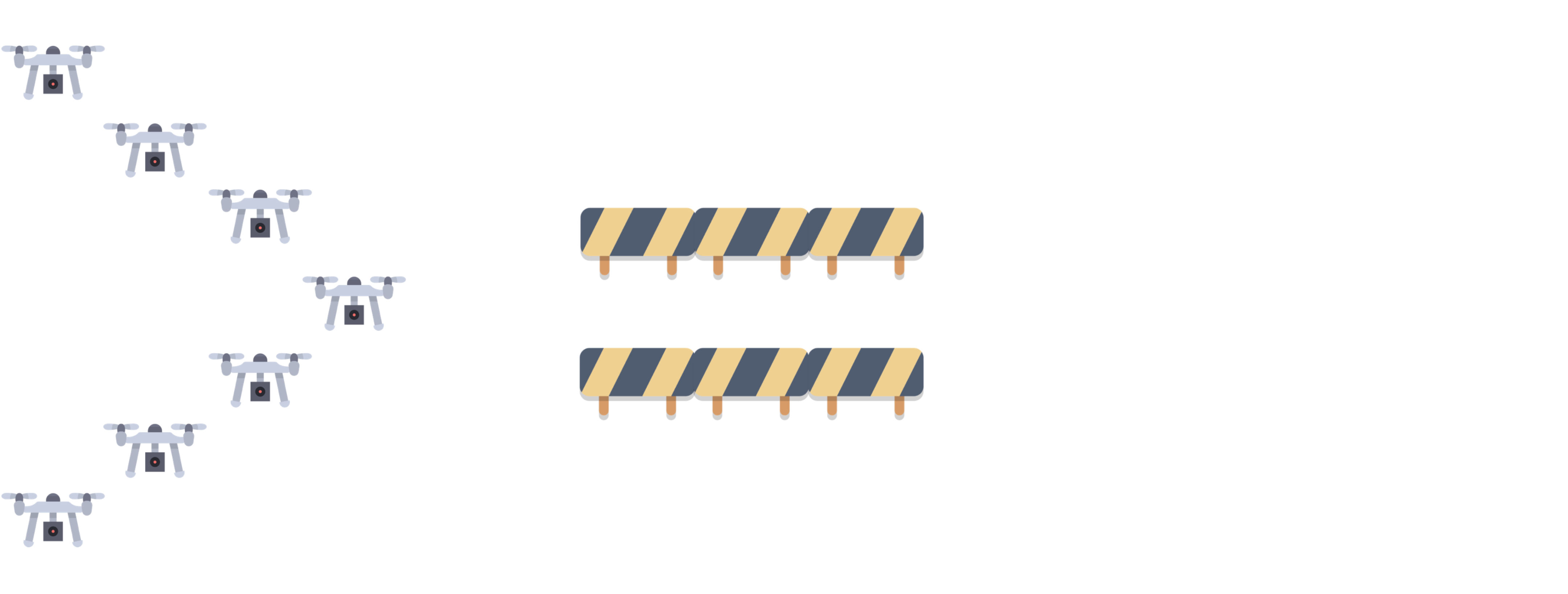
Potential issue: consistency is only eventual.
Eventual consistency
How long will it take to re-form the formation?
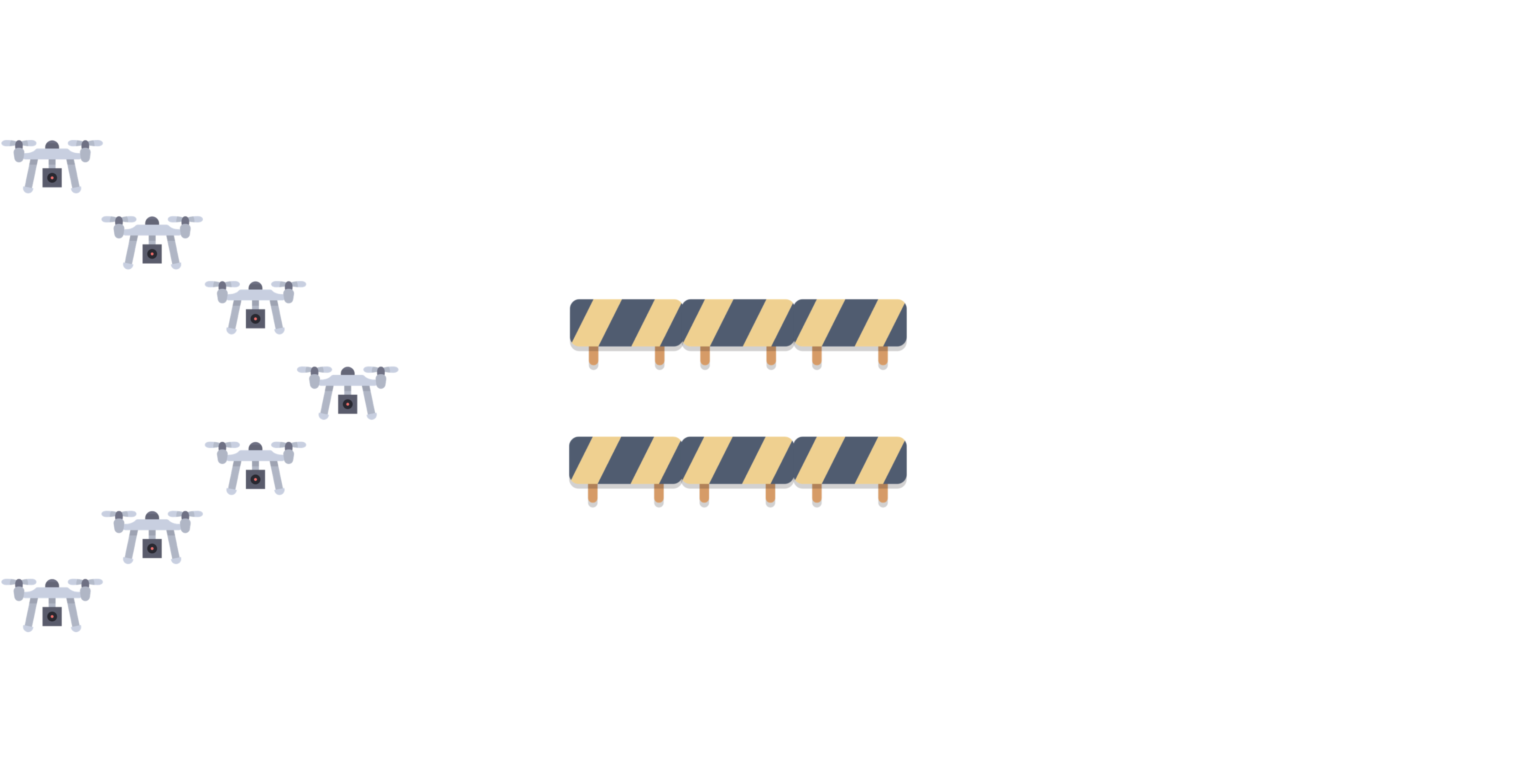
Eventual consistency
Potential issues on the transient behavior
Possible consequences of losing the formation
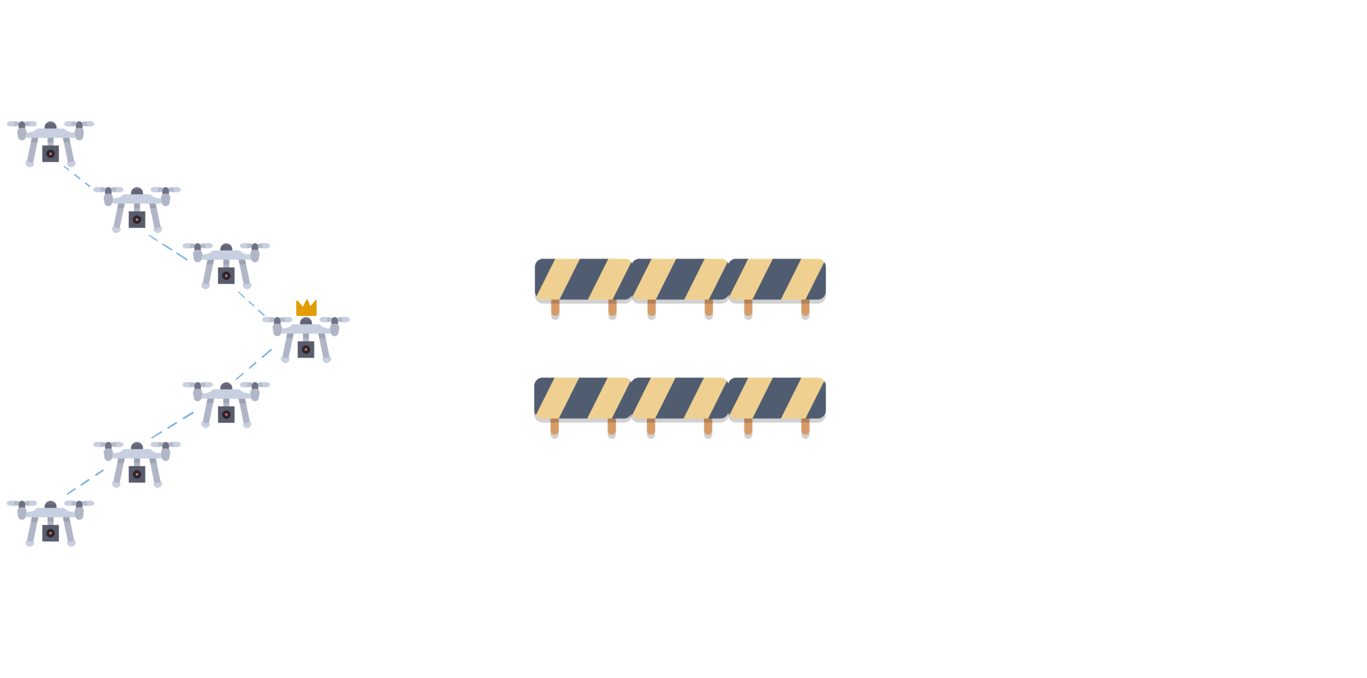
- Lost connection
- New leaders
- Sub-formations going in different directions
How we would like it to behave
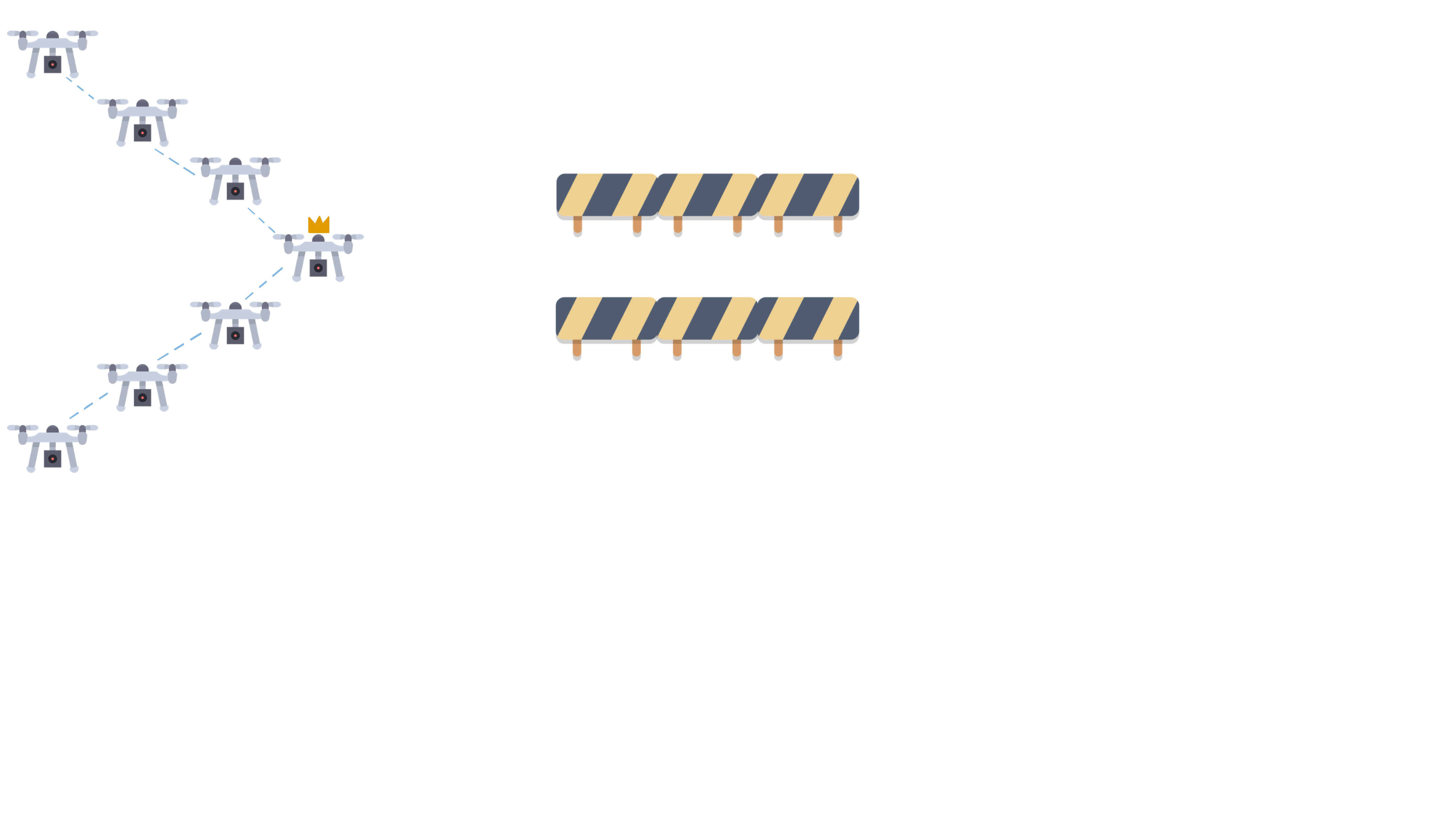
Did not lose formation, neither connection, avoided the obstacle safely and keep going towards their goal.
Our goal
Ensure guarantees on the transient behavior of the system, not only on the eventual one.
How can we achieve it?
In control theory, there exist formal methods to specify both stability and safety conditions:
- Control Lyapunov Functions (CLF) for fast convergence and stability;
- Control Barrier Functions (CBF) for safety in the transient behavior.
Preliminaries: Control Theory
Control Theory is a branch of engineering and mathematics that deals with the behavior of dynamical systems with inputs (controls).
The main goal is to develop control strategies that modify the system’s behavior to achieve a desired state,
while minimizing delays or errors, while ensuring safety and control stability.
Control can only be applied with respect to the system’s temporal evolution.
A Control Loop is a feedback-driven mechanism that measures the current state of a system,
compares it to a desired set-point,
and automatically adjusts the control input to minimize the error between the two.
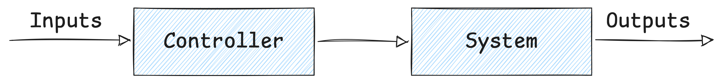
Preliminaries: Open and closed loop controls
An automatic control system can operate in two ways: as an open-loop control or as a feedback (closed-loop) control.
Open-Loop Control
The control input is determined without considering the current state of the system.
It relies on predefined control actions based on a model of the system.
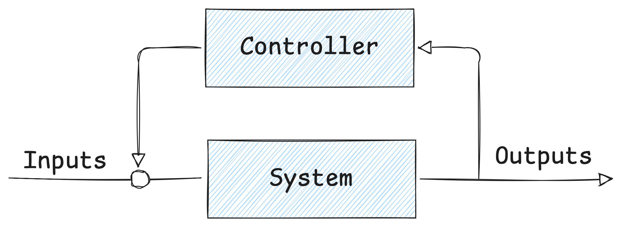
Feedback / Closed-Loop Control
The control input is continuously adjusted based on the current state of the system.
It uses feedback from the system to correct deviations from the desired state.
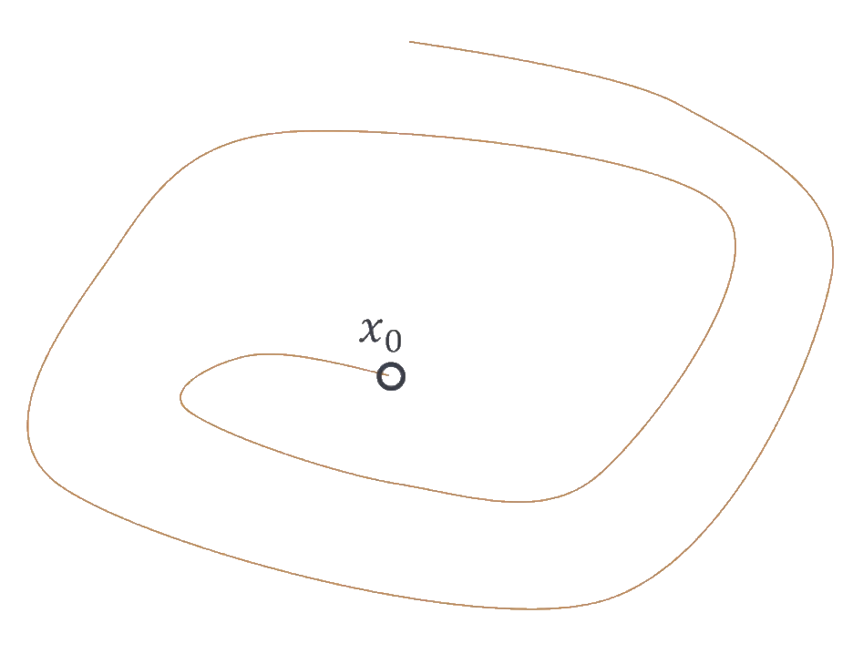
Preliminaries: Lyapunov Theory
Lyapunov Theory provides tools to analyze the stability property of dynamical systems.
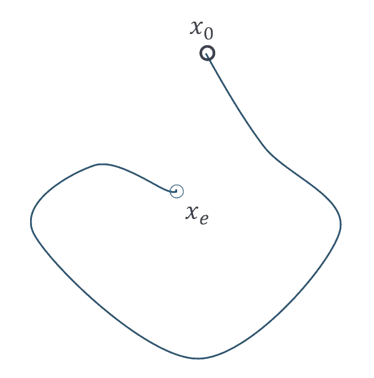
An autonomous dynamical system without a control input is described by the equation
$\dot{x} = f(x)$
Starting from an initial state $x_0$, there exist some trajectory from there, and we want to verify whether the system converges to a desired equilibrium point $x_e$.
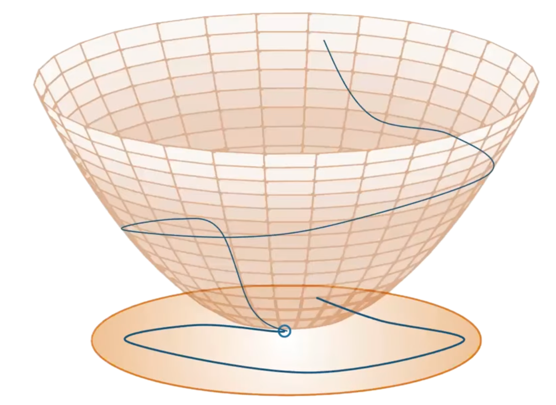
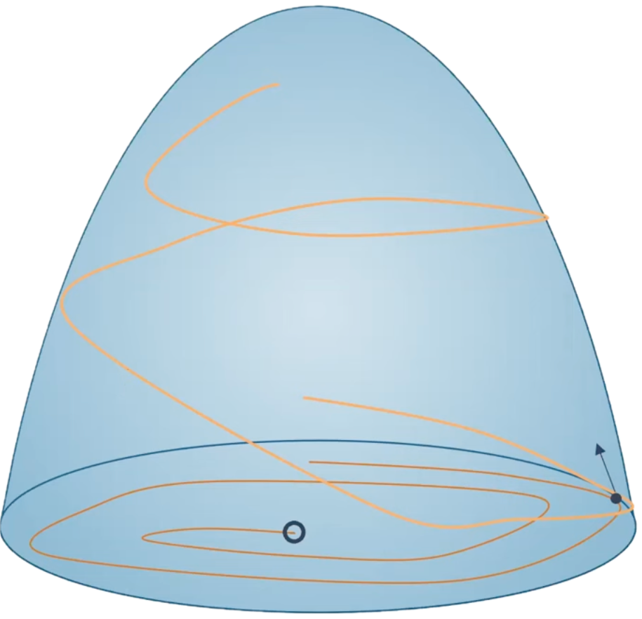
Preliminaries: Lyapunov Theory
The evolution of the function over time decreases towards $x_e$, implying that the system is stable and will converge to the desired equilibrium point. $V(x)$ is a Lyapunov Function if satisfies:
- $s.t. V(x_e) = 0, V(x) > 0 \quad \forall \quad x \neq x_e$,
- $\dot{V}(x) = \frac{\partial V}{\partial x} f(x) < 0 \quad \forall \quad x \neq x_e$,
Preliminaries: Nagumo’s Invariance Theorem
Given a different function $\dot{x} = f(x)$ and a different trajectory:
Our goal is to ensure that the trajectory remains within a region of interest.
Preliminaries: Nagumo’s Invariance Theorem
→ the set of states where the system is considered safe, also called super zero level set of $h$. To guarantee that trajectories never leave $\mathcal{C}$ (safety), it is enough to ensure that, on its boundary:
$\dot{h}(x) \geq 0 \; \forall x \in \partial \mathcal{C}$
If the condition holds, $\mathcal{C}$ is forward invariant: once inside, the system will always remain inside the safe region.
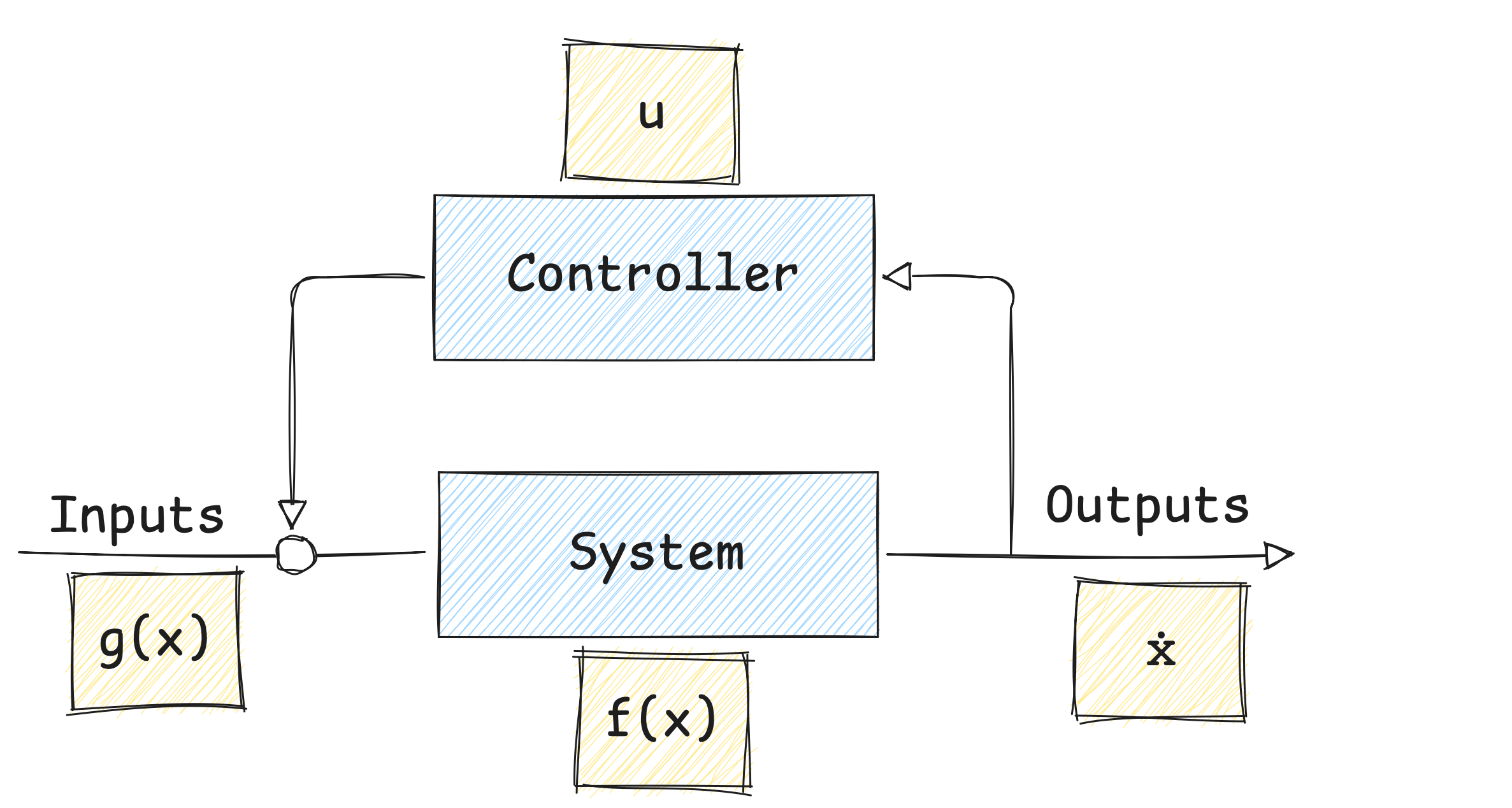
Preliminaries: Control-Affine Systems
A Control-Affine System is a dynamical system described by the equation:
$\dot{x} = f(x) + g(x)u$
where:
- $x \in \mathbb{R}^n$ is the state vector (position, velocity, etc.),
- $u \in \mathcal{U} \subset \mathbb{R}^m$ is the control input (input, actuator commands, etc.),
- $f: \mathbb{R}^n \to \mathbb{R}^n$ is the drift vector field (the natural evolution of the system without control),
- $g: \mathbb{R}^n \to \mathbb{R}^{n \times m}$ is the control input matrix (how the control input affects the system).
Preliminaries: Lie Derivatives
The Lie Derivative represents how a scalar function $h(x)$ changes in time as the state evolves,
according to the system dynamics along a vector field $f: \mathbb{R}^n \to \mathbb{R}^n$.
It is represented as $L_f h(x)$
For a Control-Affine System $\dot{x} = f(x) + g(x)u$, the time derivative of $h(x)$ is:
$\dot{h}(x, u) = L_f h(x) + L_g h(x) u$
where:
- $L_f h(x)$ is the Lie Derivative of $h$ along $f$ (drift term),
- $L_g h(x)$ is the Lie Derivative of $h$ along $g$ (control term),
- $u$ is the control input.
This notation captures how $h(x)$ evolves due to both natural dynamics and control input over time.
Control Lyapunov Functions (CLF)
A Control Lyapunov Function (CLF) is a scalar function that measures how “far” the system’s state is from a desired target set $\mathcal{X}_d$.
If we can design such a function so that it always decreases along the trajectories of the system,
then the state is driven towards $\mathcal{X}_d$ and the system can be stabilized by a suitable feedback control.
A continuously differentiable function $V: \mathbb{R}^n \to \mathbb{R}_{\geq 0}$ is a CLF for the target set $\mathcal{X}_d \subseteq \mathbb{R}^n$ if:
- $V(x) = 0 \quad \forall x \in \mathcal{X}_d$ and $V(x) > 0 \quad \forall x \notin \mathcal{X}_d$ (positive definiteness);
- $\forall x \notin \mathcal{X}_d$, there exists a control input $u \in \mathcal{U}$ and a constant $c > 0$ * such that:
$L_f V(x) + L_g V(x) u \leq -cV(x)$
CLF Example: point stabilization
For a system $\dot{p} = u$ where we want to stabilize the position $p$ of a point at a desired location $p_d$.
We want to design a control input $u$ that drives $p$ towards $p_d$.
We then define:
- the CLF: $V(p) = || p - p_d ||^2$
- the Lie Derivatives of $V$ along $f$ and $g$ respectively: $L_f V(p)=0$ $L_g V(p) = 2(p - p_d)$
Thus, $\dot{V}(p,u)=2(p-p_d)^\top u$ which links the control input $u$ to the rate of change of $V$.
Choosing a control input $u$ such that:
$u=-k(p-p_d)$ for some $k > 0$ ensures that $\dot{V} = -2k || p - p_d ||^2 \leq 0$
Which guarantees that $V(p)$ decreases exponentially over time, driving $p$ towards $p_d$ and stabilizing the system at the desired point.
Control Barrier Functions (CBF)
A Control Barrier Function (CBF) is a scalar function that defines a safe set $\mathcal{C}$
within which the system’s state must remain to ensure safety.
We want $\mathcal{C}$ to be forward invariant, i.e., if the system starts or enters in $\mathcal{C}$, it remains in $\mathcal{C}$ for all future time.
A continuously differentiable function $h: \mathbb{R}^n \to \mathbb{R}$ is a CBF for
$\mathcal{C} = \{ x \mid h(x) \geq 0 \}$
Let $\alpha$ be an extended class-$\mathcal{K}$ function (continuous, strictly increasing, $\alpha(0)=0$).
$\alpha$ acts like a safety buffer: it limits how fast $h(x)$ can decrease,
so once the system is in the safe region, it is prevented from crossing the safety boundary.
Thus, if there exists $u \in \mathcal{U}$ such that:
$L_f h(x) + L_g h(x) u + \alpha(h(x)) \ge 0 \quad \forall x \in \mathcal{D} \supset \mathcal{C}$.
Then $\dot{h}(x,u) \ge -\alpha(h(x))$
CBF Example: collision avoidance
For two agents $i, j$ with positions $p_i, p_j \in \mathbb{R}^d$, we define:
$h_{ij}(p) = || p_i - p_j ||^2 - D^2$ where $D$ is the minimum safe distance between them.
The safe set is: $\mathcal{C}_{ij} = \{ p \mid h_{ij}(p) \geq 0 \}$
Then we’ll compute the Lie Derivatives of $h_{ij}$ along $f$ and $g$ respectively:
$L_f h_{ij}(p) = 0$, $L_g h_{ij}(p)[u_i;u_j] = 2(p_i - p_j)^\top(u_i-u_j)$
To ensure collision avoidance, we need to find control inputs $u_i, u_j$ such that:
$2(p_i - p_j)^\top(u_i-u_j) + \alpha(h_{ij}(p)) \geq 0$
CLF-CBF-Quadratic Program
To get a control input that satisfies both CLF and CBF conditions,
in order to enforce both stability and safety,
we can use them as constraints in a quadratic optimization problem.
$\underset{u,s \ge 0}{\min} || u - u_{des} || + ws^2$
$s.t. \quad L_f V(x) + L_g V(x)u \leq -c V(x) + s$,
$L_f h_\ell(x) + L_g h_\ell(x) u + \alpha(h_\ell(x)) \ge 0 \quad \forall \ell$
Where:
- $u_{des}$ is a desired control input in the absence of constraints;
- $s$ is a slack variable to relax the CLF constraint when necessary (to prioritize safety);
- $w$ is a weight to penalize the slack variable;
- $\ell$ indexes multiple CBF constraints.
The CLF is softened to ensure feasibility, while CBFs are enforced strictly to guarantee safety.
The QP is solved at each time step to compute the control input $u$ that balances stability and safety,
while minimizing deviation from the desired input.
Research question(s)
- How to integrate CLF and CBF in Aggregate Computing?
- How to specify safety-critical requirements both at the single and the collective level?
- How to enforce safety and stability guarantees during the transient behavior of distributed adaptive systems?
How to integrate CLF and CBF in AC?
- Use AC to define the desired collective behavior and objectives, as usual;
- Collect neighbor information and local states at each device;
- Formulate local CLF and CBF conditions based on the collective objectives and safety requirements;
- At each device, solve a local QP that incorporates the CLF and CBF constraints to compute the control input;
- Apply the computed control input to the device’s actuators;
- Broadcast the control input and state information to neighbors for the next round of computationl.
Overview
Benefits of the integration
- Formal specification of safety and stability requirements at the collective level.
- Making safety-critical guarantees an integral part of the Aggregate Computing model.
- Safety and convergence are enforced by QP solvers at each device, ensuring local adherence to global requirements.
- Possible guarantees on transient behavior, not only eventual consistency.
Possible challenges-limitations
- Computational overhead of solving QPs on resource-constrained devices.
- Asynchrony and communication delays must be considered in the control design.
Aggregate Computing + CLF + CBF use cases
Guarantees on transient behavior in safety-critical scenarios, e.g.:
- Obstacle avoidance while maintaining formation;
- Collision avoidance between agents;
- Safe navigation in dynamic environments;
- Staying inside a designated area;
- Maintaining sufficient network connectivity;
- Respecting density limits in regions of interest.